Analysis
Analysis
First I created a statistic for the percentage of headers won, by dividing the numbers of aerials won, by the amount of headers the players engaged in. The total number of headers the players engaged in are calculated by the sum of aerials players won and players lost.
headers <- aerial_won /(aerial_lost+aerial_won)I then obtian a summary of the headers statistic, and find that there are 44 NAs. These NAs represents the number of players who have engaged in 0 aerial challenges during the 2016/2-17 premier league season.
summary(headers)## Min. 1st Qu. Median Mean 3rd Qu. Max. NA's
## 0.0000 0.3636 0.4918 0.4696 0.5952 1.0000 44Doing an intial analysis of the scatterplot graph of the statistic “headers” and the players’ height, we can see that there seems to be a positive linear correlation between the two variable.
plot(headers~height)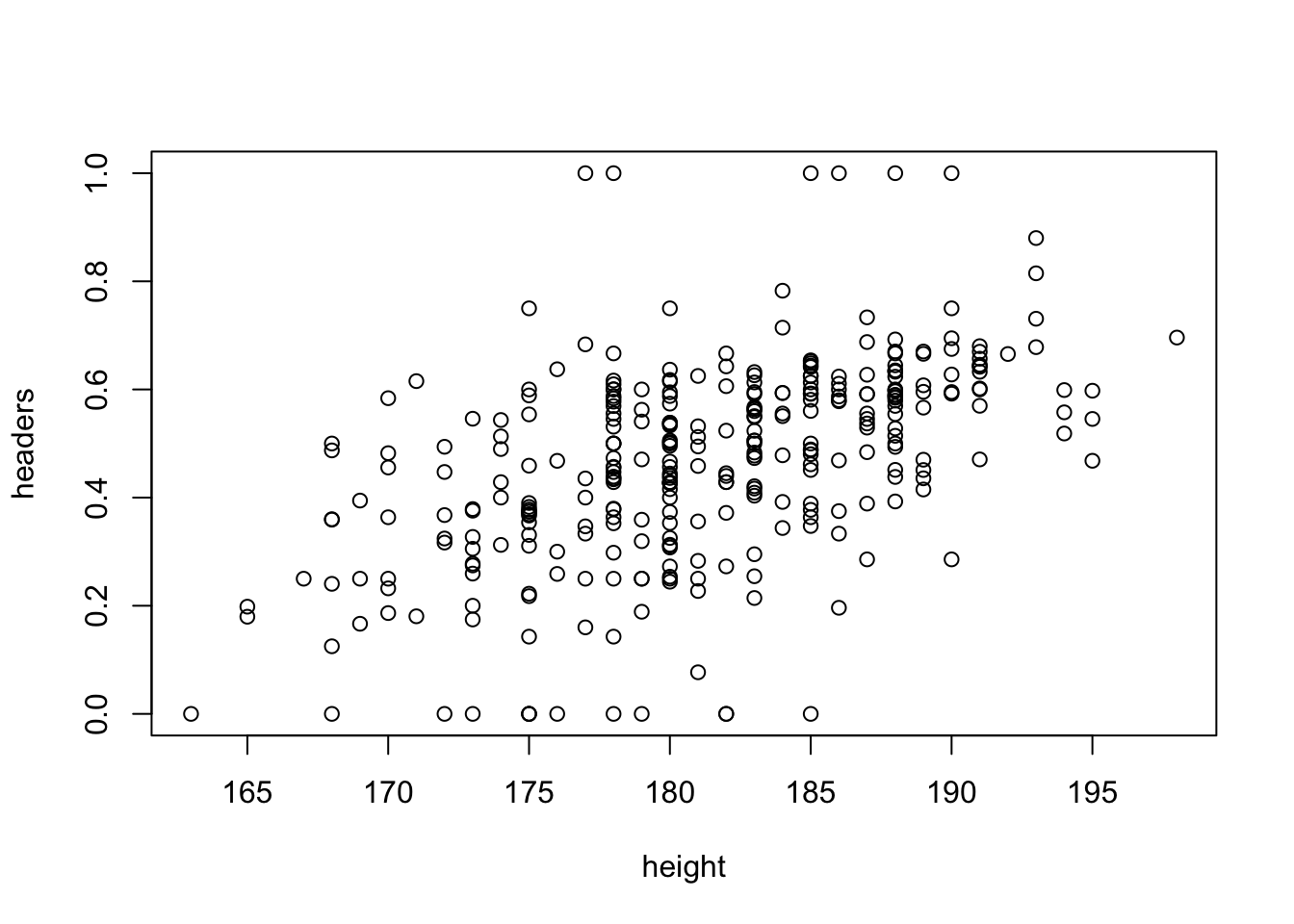
Upon a deeper analysis of this relationship, we can see that there are significant evidence that height and headers are indeed correlated, at a significance level close to 0, with a correlation of 0.015. That means that for 1 cm of height, the associated increase % of headers won is about 1.5%.
summary(lm(headers~height))##
## Call:
## lm(formula = headers ~ height)
##
## Residuals:
## Min 1Q Median 3Q Max
## -0.52509 -0.07644 0.01049 0.08447 0.59523
##
## Coefficients:
## Estimate Std. Error t value Pr(>|t|)
## (Intercept) -2.257360 0.247780 -9.11 <2e-16 ***
## height 0.015040 0.001366 11.01 <2e-16 ***
## ---
## Signif. codes: 0 '***' 0.001 '**' 0.01 '*' 0.05 '.' 0.1 ' ' 1
##
## Residual standard error: 0.1587 on 326 degrees of freedom
## (44 observations deleted due to missingness)
## Multiple R-squared: 0.2711, Adjusted R-squared: 0.2689
## F-statistic: 121.3 on 1 and 326 DF, p-value: < 2.2e-16Midfielders are normally considered to be shorter than strikers and defenders, the ability to challenge for balls are more valued in the strikers and defender positions, as they can more effiiently be turned into goals or defensive clearances. Therefore there is a possibility that it is one of the positions that is dragging the significance up. To better decipher this, I identified the correlation between the headers and height, after categorizing players by position. (Defenders = 1, Midfielders = 2, Forwards = 3)
cor(headers[position == 3], height[position == 3], use = "pairwise.complete.obs")## [1] 0.5279464cor(headers[position == 2], height[position == 2], use = "pairwise.complete.obs")## [1] 0.374691cor(headers[position == 1], height[position == 1], use = "pairwise.complete.obs")## [1] 0.4202176There seem to be a fair amount of differences with the correlation between height and headers amount the position categories. As suspected, the correlation is highest among strikers at 0.5279464, then defenders at 0.4202176 and then midfielders is the lowest at 0.374691. To find a deeper analysis, I used position as a factor variable along with height to predict the amount of headers won as well as conducted linear regression analysis within each category.
summary(lm(headers[position== 1] ~ height[position ==1]))##
## Call:
## lm(formula = headers[position == 1] ~ height[position == 1])
##
## Residuals:
## Min 1Q Median 3Q Max
## -0.45147 -0.06897 0.00326 0.06216 0.48822
##
## Coefficients:
## Estimate Std. Error t value Pr(>|t|)
## (Intercept) -1.277343 0.336208 -3.799 0.000215 ***
## height[position == 1] 0.010051 0.001828 5.499 1.74e-07 ***
## ---
## Signif. codes: 0 '***' 0.001 '**' 0.01 '*' 0.05 '.' 0.1 ' ' 1
##
## Residual standard error: 0.1289 on 141 degrees of freedom
## (21 observations deleted due to missingness)
## Multiple R-squared: 0.1766, Adjusted R-squared: 0.1707
## F-statistic: 30.24 on 1 and 141 DF, p-value: 1.742e-07summary(lm(headers[position== 2] ~ height[position ==2]))##
## Call:
## lm(formula = headers[position == 2] ~ height[position == 2])
##
## Residuals:
## Min 1Q Median 3Q Max
## -0.47658 -0.06545 0.00570 0.08422 0.60628
##
## Coefficients:
## Estimate Std. Error t value Pr(>|t|)
## (Intercept) -1.439448 0.395736 -3.637 0.00039 ***
## height[position == 2] 0.010357 0.002198 4.713 5.96e-06 ***
## ---
## Signif. codes: 0 '***' 0.001 '**' 0.01 '*' 0.05 '.' 0.1 ' ' 1
##
## Residual standard error: 0.1572 on 136 degrees of freedom
## (18 observations deleted due to missingness)
## Multiple R-squared: 0.1404, Adjusted R-squared: 0.1341
## F-statistic: 22.21 on 1 and 136 DF, p-value: 5.964e-06summary(lm(headers[position== 3] ~ height[position ==3]))##
## Call:
## lm(formula = headers[position == 3] ~ height[position == 3])
##
## Residuals:
## Min 1Q Median 3Q Max
## -0.36361 -0.06485 -0.01409 0.08391 0.30306
##
## Coefficients:
## Estimate Std. Error t value Pr(>|t|)
## (Intercept) -2.433790 0.654704 -3.717 0.000555 ***
## height[position == 3] 0.015370 0.003686 4.170 0.000137 ***
## ---
## Signif. codes: 0 '***' 0.001 '**' 0.01 '*' 0.05 '.' 0.1 ' ' 1
##
## Residual standard error: 0.1465 on 45 degrees of freedom
## (5 observations deleted due to missingness)
## Multiple R-squared: 0.2787, Adjusted R-squared: 0.2627
## F-statistic: 17.39 on 1 and 45 DF, p-value: 0.0001368summary(lm(headers ~ height* factor(position)))##
## Call:
## lm(formula = headers ~ height * factor(position))
##
## Residuals:
## Min 1Q Median 3Q Max
## -0.47658 -0.06711 0.00346 0.07198 0.60628
##
## Coefficients:
## Estimate Std. Error t value Pr(>|t|)
## (Intercept) -1.2773434 0.3754118 -3.403 0.000752 ***
## height 0.0100513 0.0020410 4.925 1.35e-06 ***
## factor(position)2 -0.1621043 0.5217100 -0.311 0.756217
## factor(position)3 -1.1564464 0.7446853 -1.553 0.121421
## height:factor(position)2 0.0003056 0.0028658 0.107 0.915135
## height:factor(position)3 0.0053191 0.0041564 1.280 0.201557
## ---
## Signif. codes: 0 '***' 0.001 '**' 0.01 '*' 0.05 '.' 0.1 ' ' 1
##
## Residual standard error: 0.1439 on 322 degrees of freedom
## (44 observations deleted due to missingness)
## Multiple R-squared: 0.4079, Adjusted R-squared: 0.3987
## F-statistic: 44.36 on 5 and 322 DF, p-value: < 2.2e-16Through the within category linear regression anlysis, we can see that the difference is slight, only at about 0.0005 difference in correlation between the defenders and forwards. This is confirmed by using position as a factor variable. While the height is still a significant variable, it does not seem that the position introduced a significant effect into the equation, as neither a factor variable nor as a interaction coefficient with height.
Fans often argue that players need adaptaion into the first team playing, particularly a competitive league like the premier league. They take time to learn and show their potential. Perhaps this “learning” also applies to ability to win aerial challenges. I shall conduct a model for both the number of games played in the Premier League, their height and their headers ability.
summary(lm(headers ~ appearances + height))##
## Call:
## lm(formula = headers ~ appearances + height)
##
## Residuals:
## Min 1Q Median 3Q Max
## -0.51551 -0.08344 0.01052 0.08655 0.60529
##
## Coefficients:
## Estimate Std. Error t value Pr(>|t|)
## (Intercept) -2.271e+00 2.479e-01 -9.161 <2e-16 ***
## appearances 1.097e-04 9.184e-05 1.195 0.233
## height 1.506e-02 1.365e-03 11.032 <2e-16 ***
## ---
## Signif. codes: 0 '***' 0.001 '**' 0.01 '*' 0.05 '.' 0.1 ' ' 1
##
## Residual standard error: 0.1586 on 325 degrees of freedom
## (44 observations deleted due to missingness)
## Multiple R-squared: 0.2743, Adjusted R-squared: 0.2699
## F-statistic: 61.43 on 2 and 325 DF, p-value: < 2.2e-16As you can see here, even though learning may apply to the other aspects. It seems that the ability to win aerial challenges are not significantly affected by the number of appearance made by the individuals.
Finally I want to see if the aerial ability of strikers actually translate to a substantial increase into chances for a goal, such that it would make sense for Premier League clubs to pay a premium for taller strikers that are better at contesting in the air.
goalspg <- goals/appearances
summary(lm(goalspg ~ headers))
##
## Call:
## lm(formula = goalspg ~ headers)
##
## Residuals:
## Min 1Q Median 3Q Max
## -0.26669 -0.16549 -0.11518 -0.05718 1.01200
##
## Coefficients:
## Estimate Std. Error t value Pr(>|t|)
## (Intercept) 0.29150 0.04998 5.832 1.32e-08 ***
## headers -0.30350 0.09901 -3.065 0.00236 **
## ---
## Signif. codes: 0 '***' 0.001 '**' 0.01 '*' 0.05 '.' 0.1 ' ' 1
##
## Residual standard error: 0.3322 on 326 degrees of freedom
## (44 observations deleted due to missingness)
## Multiple R-squared: 0.02802, Adjusted R-squared: 0.02504
## F-statistic: 9.397 on 1 and 326 DF, p-value: 0.002355summary(lm(goalspg [position==3] ~ headers[position==3]))##
## Call:
## lm(formula = goalspg[position == 3] ~ headers[position == 3])
##
## Residuals:
## Min 1Q Median 3Q Max
## -0.3326 -0.2736 -0.2363 0.3125 0.8664
##
## Coefficients:
## Estimate Std. Error t value Pr(>|t|)
## (Intercept) 0.3602 0.1290 2.792 0.00766 **
## headers[position == 3] -0.3399 0.3797 -0.895 0.37541
## ---
## Signif. codes: 0 '***' 0.001 '**' 0.01 '*' 0.05 '.' 0.1 ' ' 1
##
## Residual standard error: 0.4393 on 45 degrees of freedom
## (5 observations deleted due to missingness)
## Multiple R-squared: 0.0175, Adjusted R-squared: -0.004334
## F-statistic: 0.8015 on 1 and 45 DF, p-value: 0.3754I first start by creating a new statistic for goals per game, this statistic helps me standardize in order to analyze the rate of goals influenced by the ability to win an aerial challenge. This seem to yield a significant negative correlation of the two statistic. In order to get a better idea of what this means, I narrowed the scope to just strikers
Then I analyzed a linear regression model between goals per game and the % of headers won for just attacking players (position 3). There is no significant correlation. It may also be that instead of scoring the goals from winning the aerial challenge, the striker may be providing an assist for a goal.
goalassistspg <- (goals + goal_assist)/appearances
summary(lm(goalassistspg ~ headers))
##
## Call:
## lm(formula = goalassistspg ~ headers)
##
## Residuals:
## Min 1Q Median 3Q Max
## -0.34331 -0.16709 -0.10351 -0.02678 1.05334
##
## Coefficients:
## Estimate Std. Error t value Pr(>|t|)
## (Intercept) 0.44312 0.04796 9.240 < 2e-16 ***
## headers -0.48585 0.09499 -5.115 5.37e-07 ***
## ---
## Signif. codes: 0 '***' 0.001 '**' 0.01 '*' 0.05 '.' 0.1 ' ' 1
##
## Residual standard error: 0.3188 on 326 degrees of freedom
## (44 observations deleted due to missingness)
## Multiple R-squared: 0.07428, Adjusted R-squared: 0.07144
## F-statistic: 26.16 on 1 and 326 DF, p-value: 5.375e-07summary(lm(goalassistspg [position==3] ~ headers[position==3]))##
## Call:
## lm(formula = goalassistspg[position == 3] ~ headers[position ==
## 3])
##
## Residuals:
## Min 1Q Median 3Q Max
## -0.3963 -0.2886 -0.1987 0.2331 0.9959
##
## Coefficients:
## Estimate Std. Error t value Pr(>|t|)
## (Intercept) 0.4941 0.1247 3.961 0.000263 ***
## headers[position == 3] -0.4599 0.3670 -1.253 0.216705
## ---
## Signif. codes: 0 '***' 0.001 '**' 0.01 '*' 0.05 '.' 0.1 ' ' 1
##
## Residual standard error: 0.4247 on 45 degrees of freedom
## (5 observations deleted due to missingness)
## Multiple R-squared: 0.03371, Adjusted R-squared: 0.01224
## F-statistic: 1.57 on 1 and 45 DF, p-value: 0.2167Similarly here, we can see that there is no significant correlation between goals and assists per game with the players’ heading ability for strikers, while in general we also see a negative correlation in our linear regression model. It seems that the Premier League clubs are being inefficient in the distribution of their funds when they are spending a premier to buy taller strikers, strictly in terms of the goals and assists they may provide.
plot(goalspg [position ==3] ~ headers [position ==3])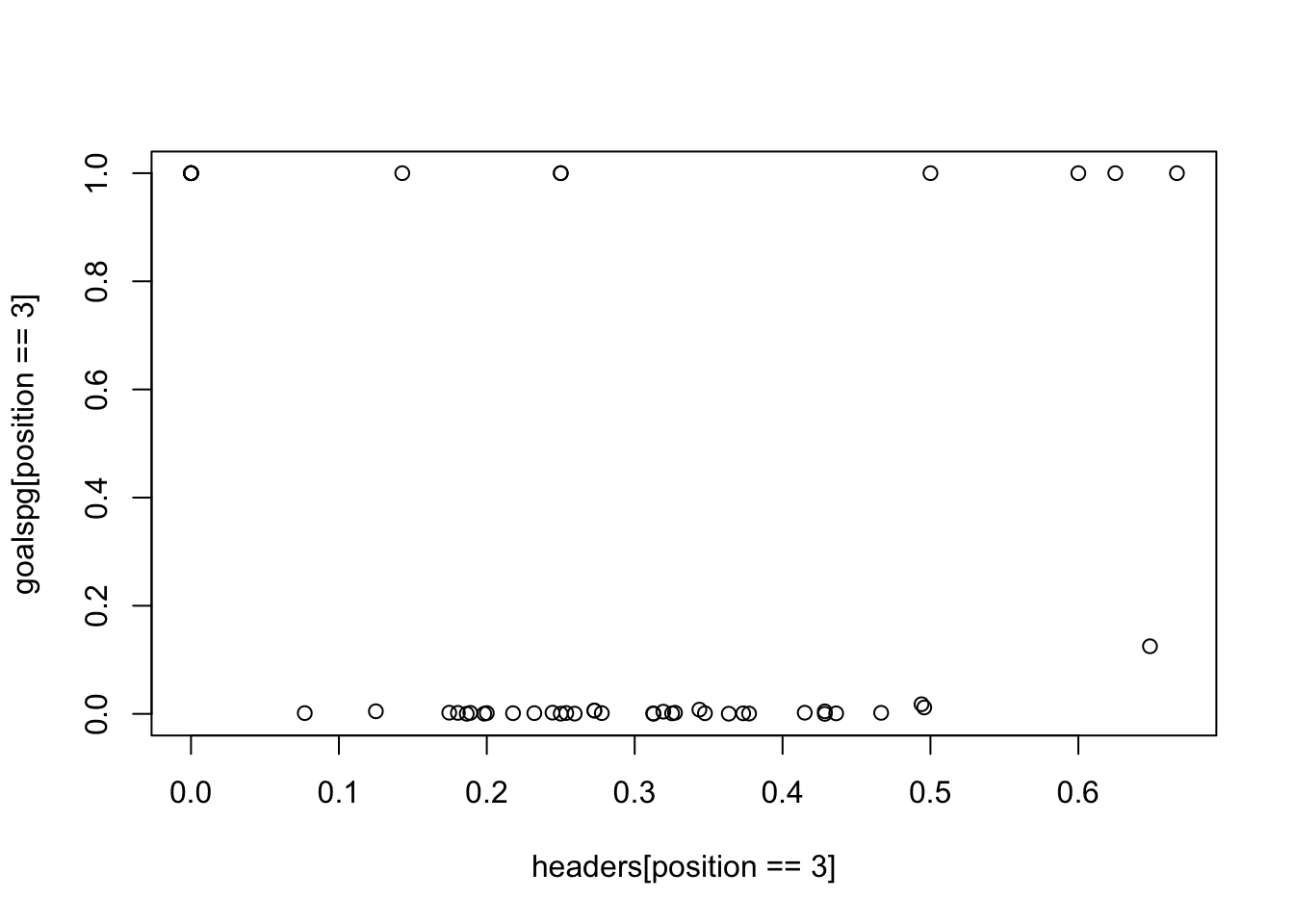
plot(goalassistspg [position ==3] ~ headers [position ==3])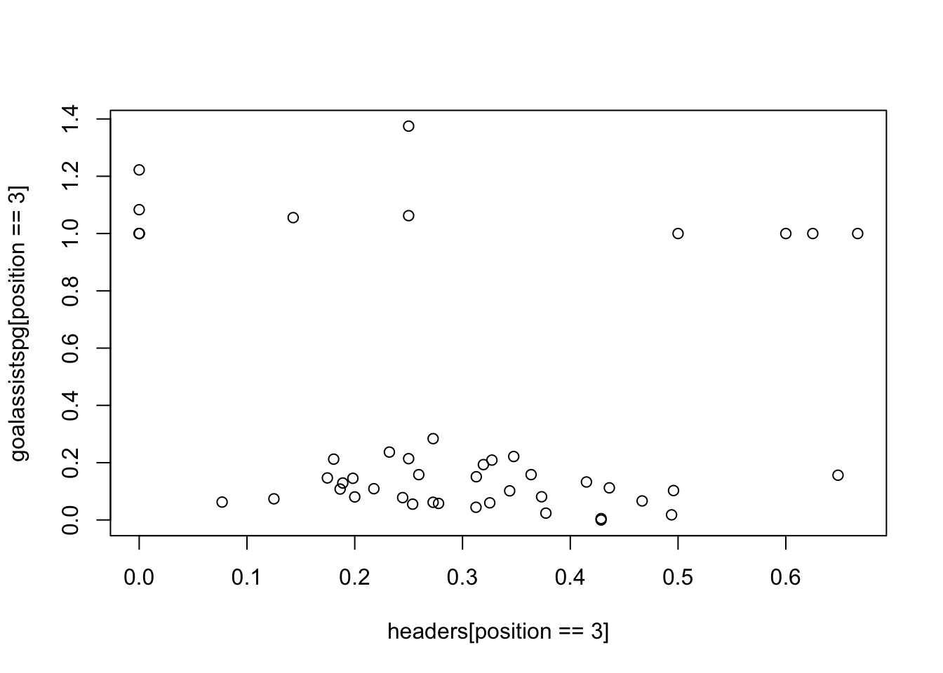
Strangely enough, when we plot the dataset, there seems to be a large divide between the two groups of attacking players. Several players are much better at translating their aerial challenges into goals and assists, whiles others’ aerial challenges result in close to no goals and assist. This may be due to the fact taht both strikers and wingers are categorized as attacking players in this dataset.